
Analysis of VPFFT for HPC
Back in 2014, during my stay in Universitat Politècnica de Catalunya (UPC), I took a course on Parallel Programming Tools and Models (PPTM) as part of the MSc syllabus. While everything seemed quite confusing at first, looking back I realize it was one of the most interesting projects I did.
The assignment: Analyze an application for deployment in the MareNostrum3 Supercomputer! Our choice, no restrictions. And we get to run it in one of the fastest supercomputers in existence! How cool is that?
However, freedom comes at a cost – finding a suitable application was no easy task. Some were inadequate for HPC, some were terribly complicated. I remember searching for several days!
I ended up choosing VPFFT++, a Crystal viscoplasticity proxy application by Exascale Co-design Center for Materials in Extreme Environments (ExMatEx).
What is VPFFT++?
VPFFT is a solver for Polycrystalline Mechanical Properties, an implementation of a mesoscale micro-mechanical materials model. VPFFT simulates the evolution of a material under deformation by solving the viscoplasticity model. The solution time to the viscoplasticity model, which is described by a set of partial differential equations, is significantly reduced by application of the Fast Fourier Transform (FFT) in the VPFFT algorithm.
VPFFT++ is a reference implementation of the algorithms in VPFFT. While capturing most of its computational complexity, VPFFT++ does not employ most of the machine-specific optimizations and additional physics feature sets from the original VPFFT code.
VPFFT++ is written in C++ and uses GNU Make to reduce external dependency requirements for building it. It is claimed to have implemented parallelization through MPI and OpenMP, though no traces of OpenMP usage were at time present in the source code.
It depends on two open source libraries:
- FFTW (“Fastest Fourier Transform in the West”) - which is probably one of the best-named pieces of software ever! - a C subroutine library for computing the Discrete Fourier Transform (DFT) in a multidimensional space, of arbitrary input size and of both real and complex data
- Eigen - a C++ template library for linear algebra: matrices, vectors, numerical solvers and related algorithms.
Very cool slides of a presentation on VPFFT++ can be found here
Full disclaimer: I never really understood what the algorithm accomplishes. I am no expert in VPFFT, nor in material modelling. My task was to just analyze the software and try to improve its efficiency in MareNostrum3.
Starting off
At the time I started the analysis, VPFFT++’s latest version only had support for OpenMP, with a hardcoded limit of 8 threads doing work. Damn! I can’t use it either, I thought. However, I got lucky! After contacting the author (a big thanks to Frankie Li from LLNL), he kindly and swiftly updated the repository with a MPI version (while at the same time dropping OpenMP support). I can live without OpenMP. Let’s give it a shot!
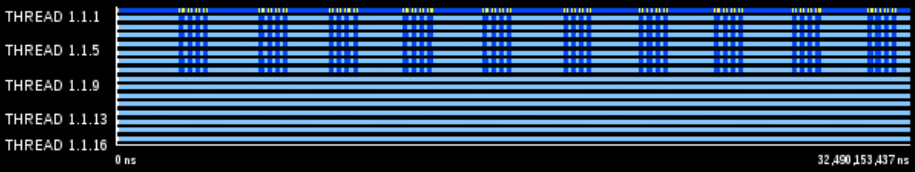 |
|---|
| First version of VPFFT++ on two nodes, one process per node, default view |
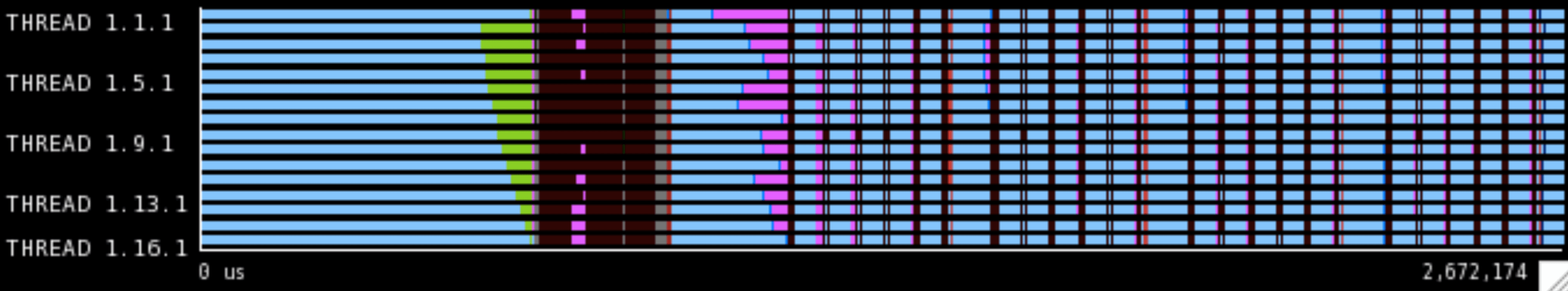 |
|---|
| Updated version of VPFFT++ on 16 nodes, one process per node, MPI calls view |
Problem Encoding
So, the problem is internally represented as a 3D matrix, and split along its X axis in equal-length chunks (that is, if the length in X axis is divisible by the number of processes), each to be assigned to a specific process. The application itself does not really accept the problem parameters upon execution - all of them are hardcoded(!), and the ones that come by default end up generating a runtime error if compiled with the debug option. However, the production version does not perform sanity checks and runs fine (although the application results might lose their significance completely).
In order to tweak the behavior of the application, several parameters that correspond to the problem to be solved must be tweaked in the source code itself:
- Matrix size: by default is
16x16x16. This was tweaked to be up to 256x256x256 due to some processes being idle at high process counts. Matrixes bigger than256x256x256are too big to fit in MareNostrum III nodes’ memory. If we require more workers, one may increase the X dimension while reducing the Y and Z lengths. This may be a problem if one requires a matrix that doesn’t fit in memory. - Number of Iterations: This indicates the number of (inner) iterations to be ran per time step. By default, the value is
100. - Number of Time Steps: The number of strain steps to simulate. This value controls how many outer iterations are performed. By default, the value is 100.
- Time Step, which is domain-specific, has a default value of
3E-2. This represents the simulation duration of each strain simulation step. It might influence the number of iterations indirectly, by influencing the result of each iteration, by lowering the iteration error (see next parameter). - Convergence Epsilon represents a lower boundary on each strain ste, which is also domain-specific. If the Stress Error or Strain Rate Error values go below this Epsilon, the strain step ends, ignoring the number of iterations aforementioned. This value is kept to its default of
10E5.
Application Structure
As stated before, the algorithm is composed of iterations at two levels - an outer loop, and an inner loop. We will call each iteration of the outer loop a time step simulation - I will use both definitions interchangeably.
The outer loop simply calls the strain step algorithm (the inner loop) a predetermined amount of times. For each time step completed, a line is written in the output file (Stress_Strain.txt).
The inner loop is slightly more complicated. Before the actual iterations there is a compute-intensive phase, followed by an MPI AllReduce communication phase - we will call this the time step initialization phase. Afterwards, it performs several iterations up to a certain predetermined maximum amount (see previous section). If it finds the stress and strain deviation from the solution (an error value) is under a convergence epsilon (see previous section), it might run less iterations.
A visual representation of this decomposition can be observed in figure 3. We see the initialization phase of the first time step lasts a lot more time and is very imbalanced. This behavior is exclusive of the first iteration. Therefore, the initialization phase of this time step is not included in the analysis. Figure 4 shows the MPI calls timeline in an execution of a single time step.
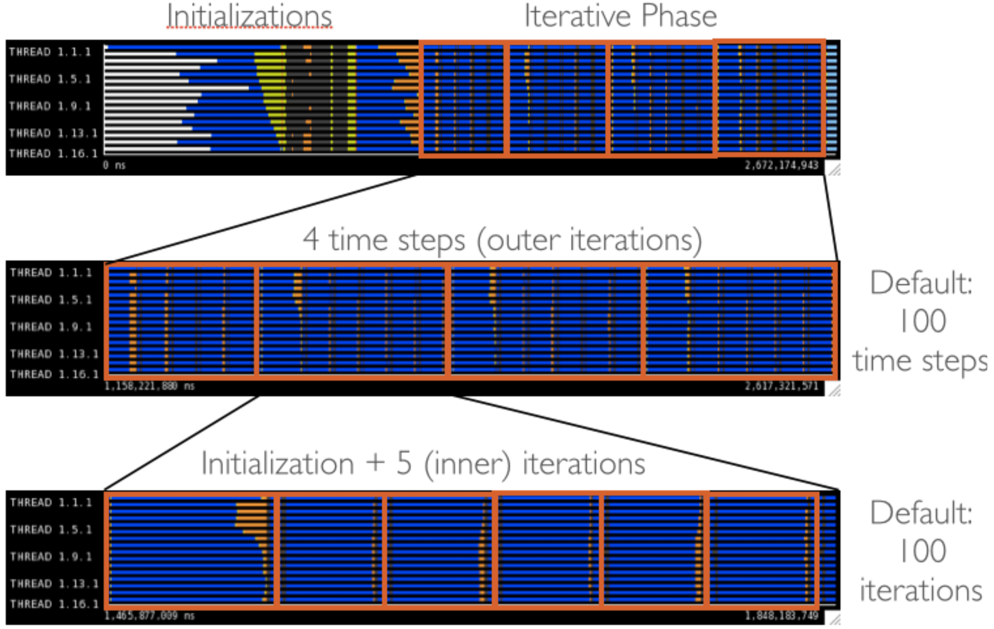 |
|---|
| Visual decomposition of the application structure using 4 outer iterations and 5 inner iterations. |
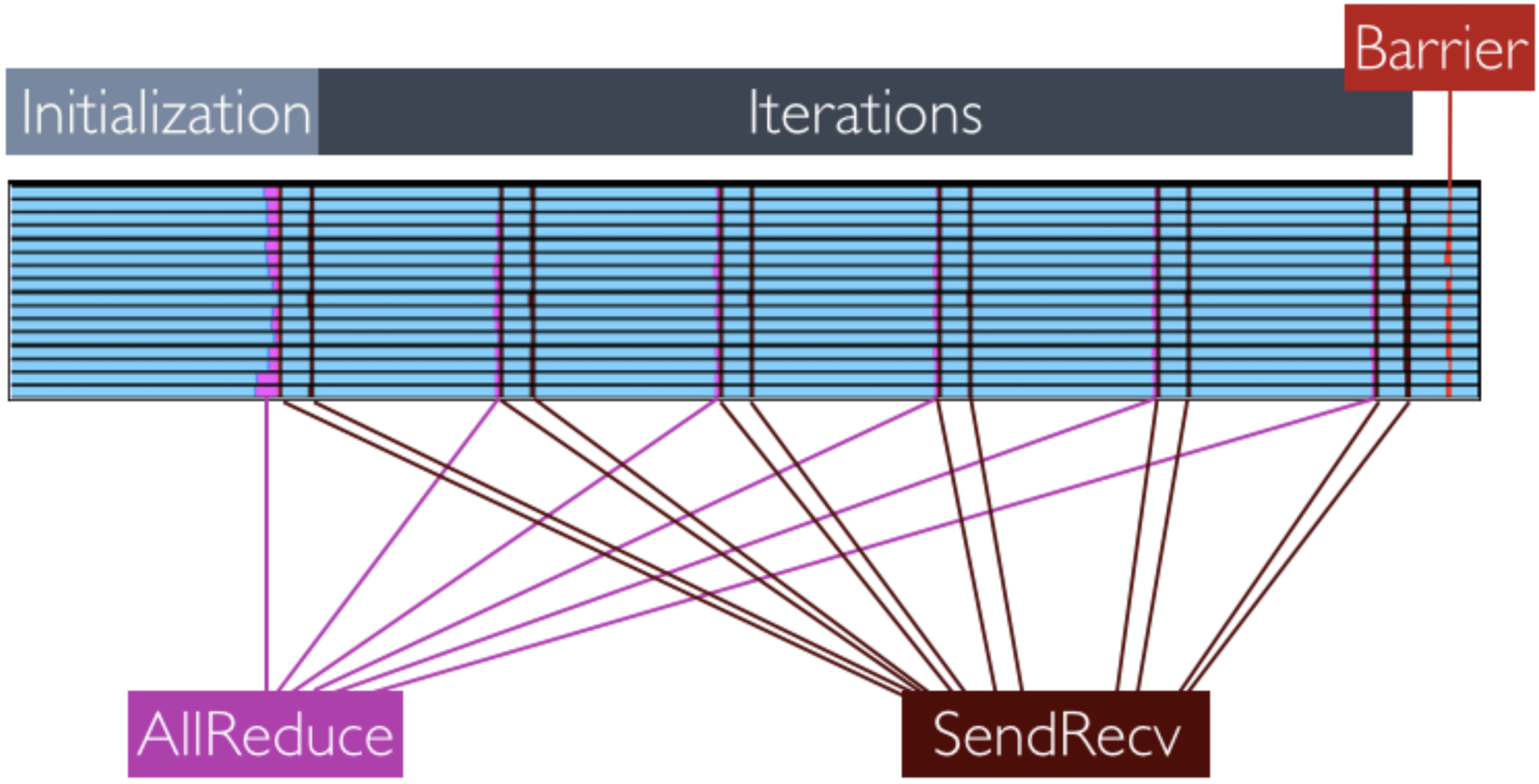 |
|---|
| Different MPI calls located within the trace of a single time step. |
Speedup and Efficiency
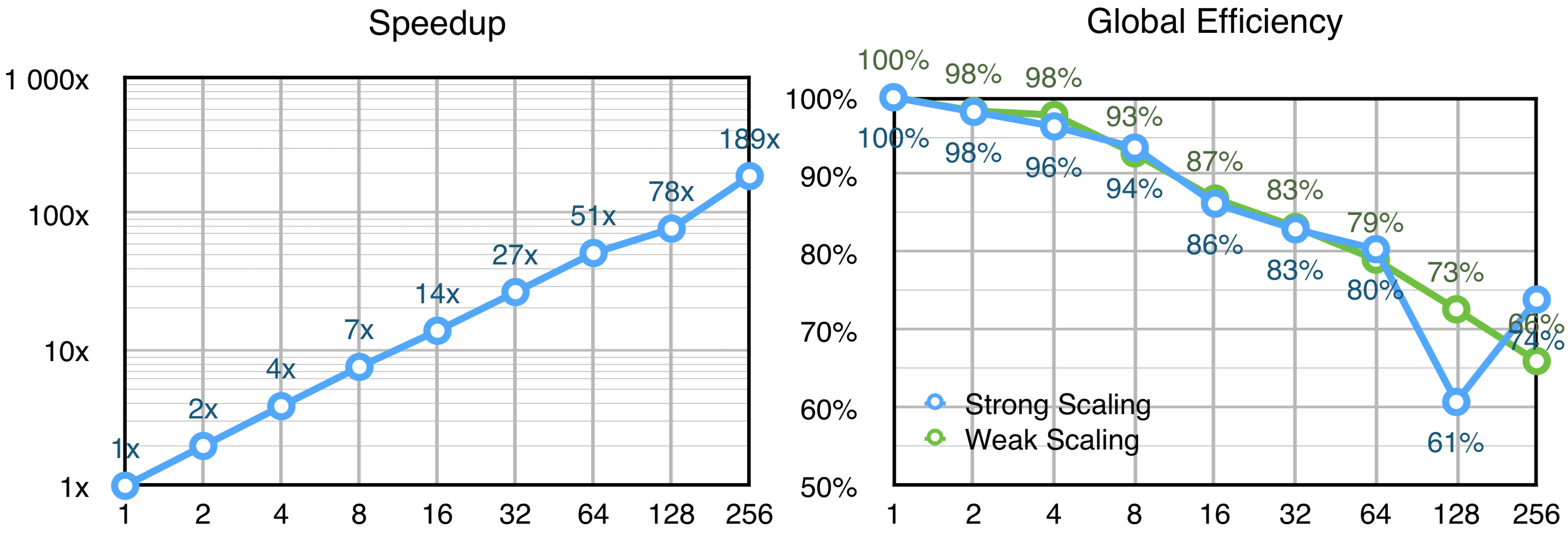
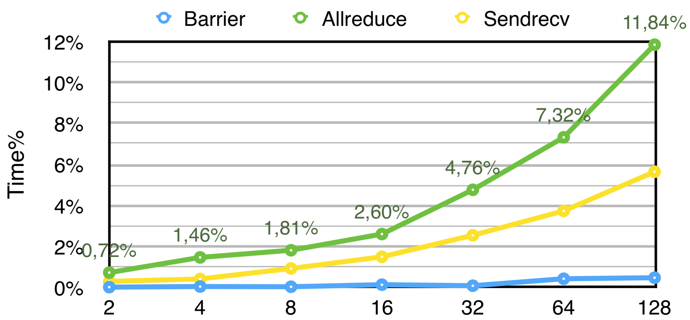
Preliminary runs on the scalability of the application reveals it scales well beyond the 16-core limitation imposed by default values, but with reduced efficiency. The results can be seen in Figure 5. The data gathered was based on the execution time reported by the application. Time spent in initializations prior to the algorithm execution is not included. Strong scaling was evaluated using 5 time steps, with 10 iterations each, using a 256x256x256 matrix. Weak scaling was evaluated using 5 time steps, with 5 iterations each, using a Nx256x256 matrix, where N denotes the number of processes used for each run. Figure 6 shows the percentage of time spent in MPI communication phases for Strong Scaling - the values were gathered from traces generated by Extrae in independent runs from those in Figure 5.
 |
|---|
| Global Speedup and Efficiency of the Application for Strong Scaling (blue) and Weak Scaling (green). The x-axis represents the number of processes. |
 |
|---|
| Percentage of time spent in MPI calls for Strong Scaling tests. The x axis represents the number of processes. |
Efficiency Model
We now present an efficiency model for analysis of VPFFT++:
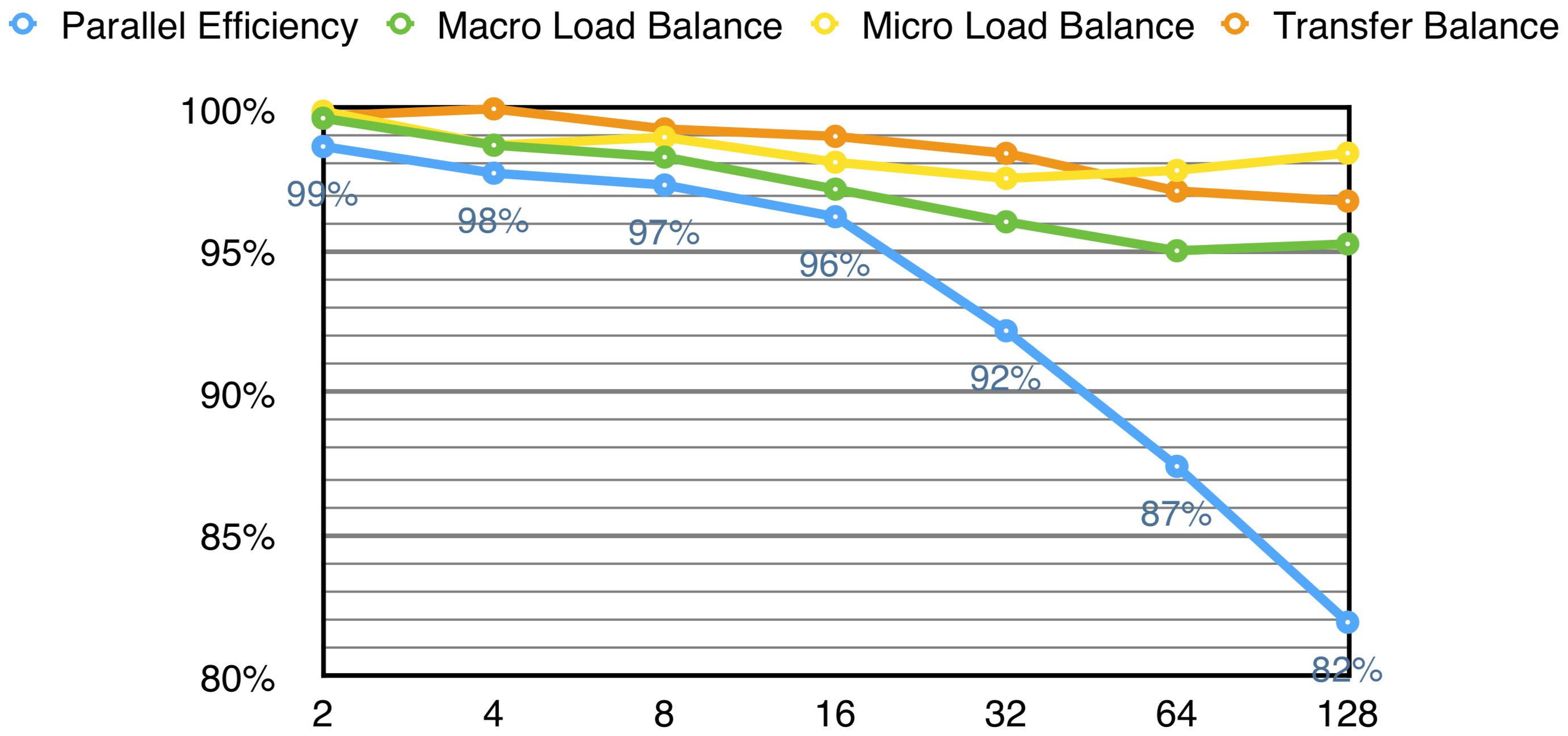
- Macro Load Balance is the maximum time a process spends doing computation, according to real world measurements.
- Micro Load Balance is the maximum time a process spends doing computation, given that the network has infinite bandwidth and zero latency. Because of the perfect network conditions, if there was no imbalance between the processes, one would expect a value of
100%. - Transfer Imbalance is the Macro Load Balance divided by the Micro Load Balance. Represents how uneven is the communication load distribution between the different processes.
- Parallel Efficiency is the average time a process spent doing computation, among all processes.
 |
|---|
| Efficiency Model for VPFFT++. The x axis represents the number of processes. |
We see the biggest cause for loss in efficiency is Macro Load Imbalance. We can see that all parameters degrade, though, and eventually each of them may become a problem by itself.
Computational Imbalance
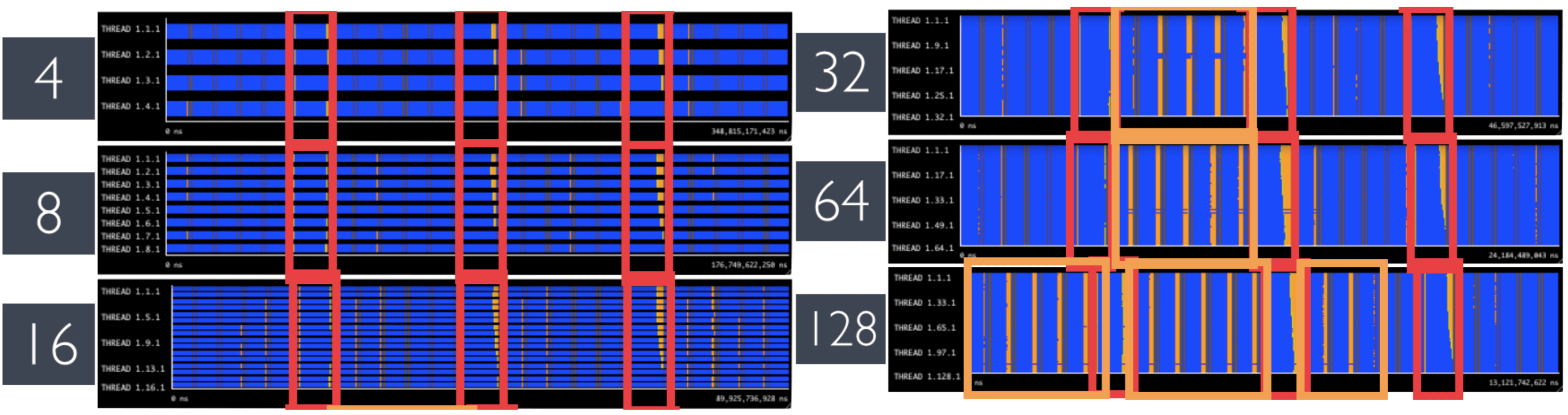
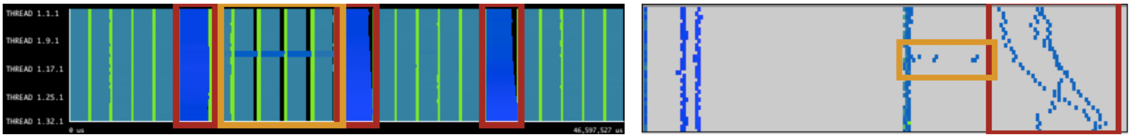
As shown before, the time step initialization phases are not well-balanced. This imbalance is deterministic, and has a slightly different pattern for each of the iterations. In Figure 8, one can see that the shape of these regions (in red) remains the same with varying number of processes. However, at higher core counts, we see there is some extra imbalance in the otherwise balanced iterations. This effect appears to be non-deterministic, and causes some processes to take extra time doing computation.
 |
|---|
| Computational Imbalance regions with 4, 8, 16, 32, 64 and 128 processes. Identified in red are periodic imbalance. In orange are identified regions where imbalance seems random. |
To gain more insight onto what causes these two regions of imbalance, the first step is to take a look at the Useful Duration. In Figure 9, one can clearly identify the same red and orange regions as before. We see that the red regions share a higher duration than all other phases of the program, and the orange region is a slight deviation in duration of two consecutive processes. It should be pointed out that these traces were gathered using 4 processes per node (which has two sockets), and both processes experiencing this variation are running on the same node.
 |
|---|
| Useful Duration for 32 processes. Left: timeline of duration of computation regions (blue is higher). On the right, the corresponding histogram in which the x-axis represents duration in a linear fashion. |
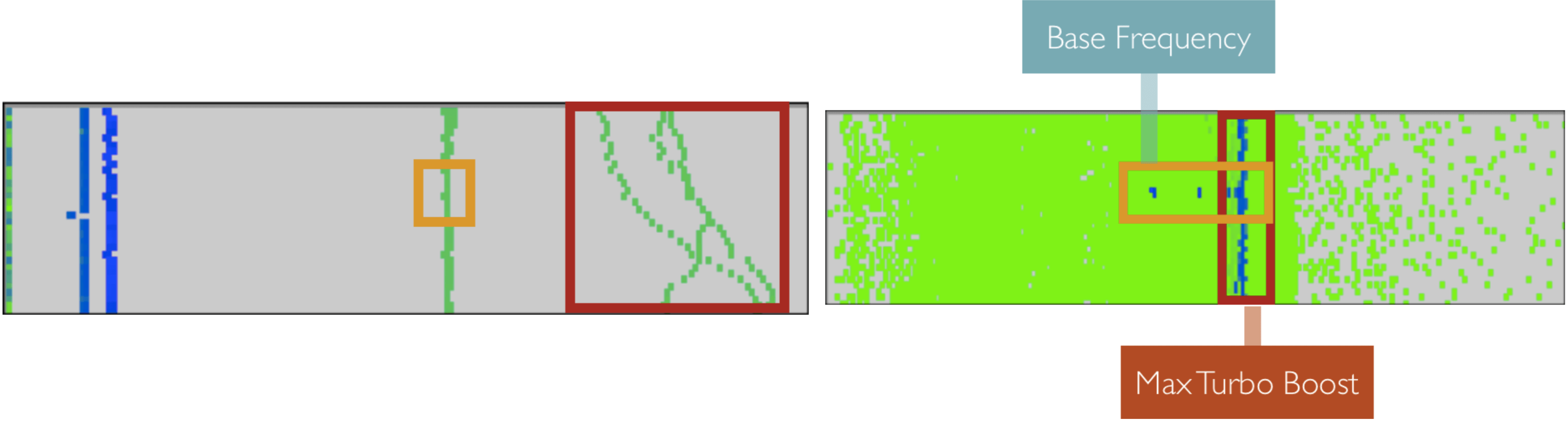
We can try to identify the causes of noise by analyzing different views from the same trace, as seen in Figure 10. The red region appears to be algorithmic, while the orange one caused by noise - a reduction in CPU frequency(!). Both processes were placed in the same CPU and TurboBoost got deactivated for a short period of time. We might be able to remove this source of noise by running more processes on a single node (which probably cause all processes to run at the normal CPU frequency), but that is outside the scope of this report.
 |
|---|
| Total instructions (left) and Cycles per µs (right) for 32 processes. |
Removing Noise
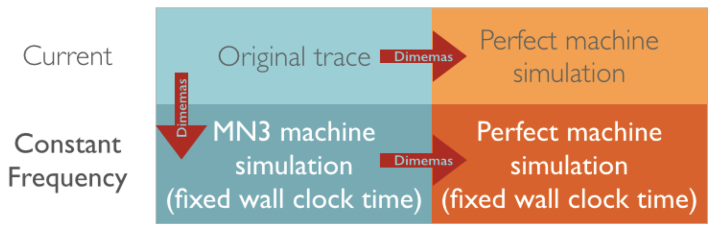
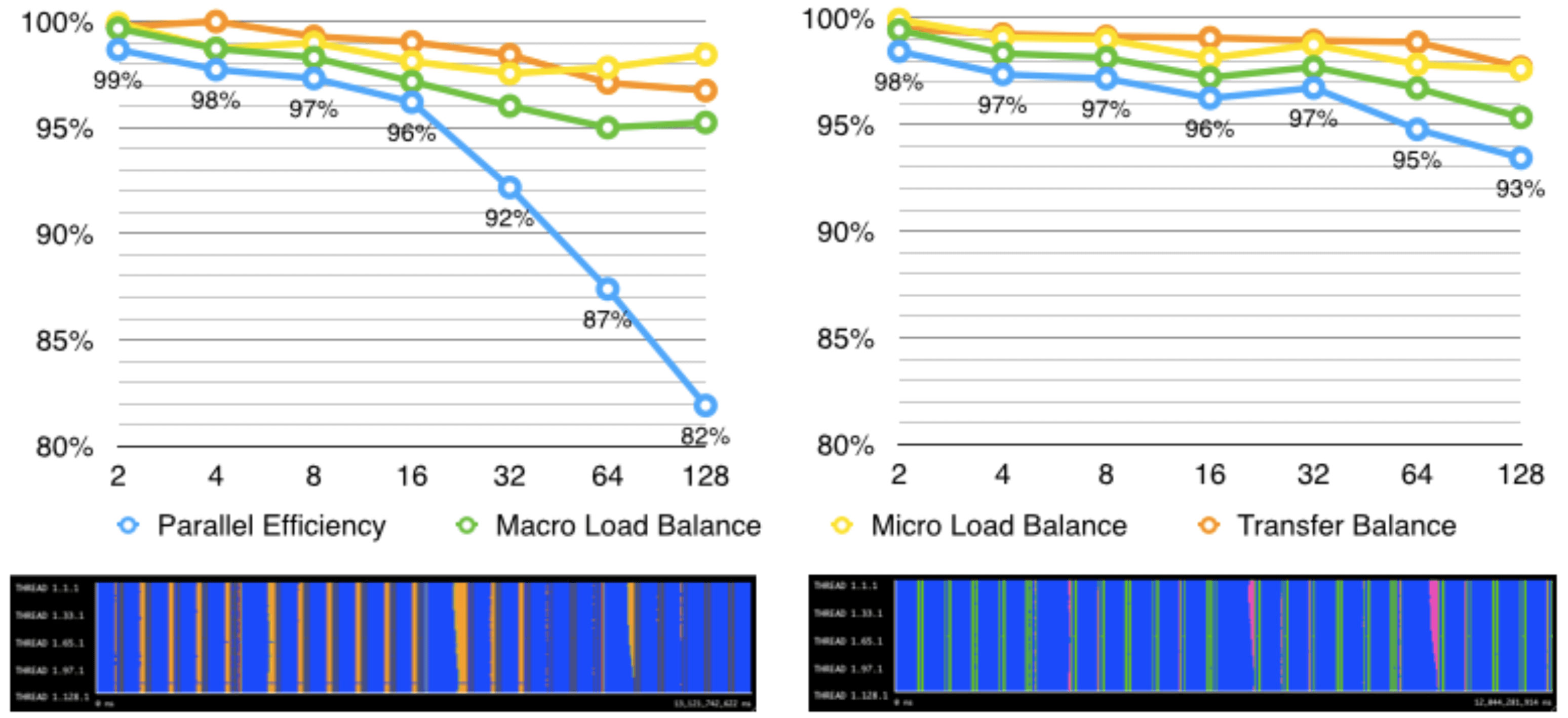
The noise caused by the seemingly innocent change in CPU frequency might be the main factor driving down the efficiency of the parallel execution. In order to determine this, we will attempt to remove the noise by simulating a constant CPU frequency (at 3.3GHz, which is the Turbo frequency for two cores being used in the CPUs used by MareNostrum III). The process is described briefly in a graphical way in Figure 11. From the original trace, we will run a Dimemas simulation where we specify a fixed CPU wall clock time. From this, we can apply the same efficiency model as before by also simulating execution with a perfect network, which is depicted in Figure 12 with a comparison against the efficiency obtained with noise. We can see there is a huge improvement in parallel efficiency where CPU noise was a problem (over 32 processes). Now we are left with no significant external noise, and the imbalance that we can see is caused by the algorithm itself.
 |
|---|
| Methodology applied to remove noise related to changes in CPU frequency |
 |
|---|
| Efficiency model for the original trace (left) and trace with a constant CPU wall clock time (right). The total time of the original is 13.121 seconds, and the simulated trace is 12.044 seconds. |
Algorithmic Imbalance
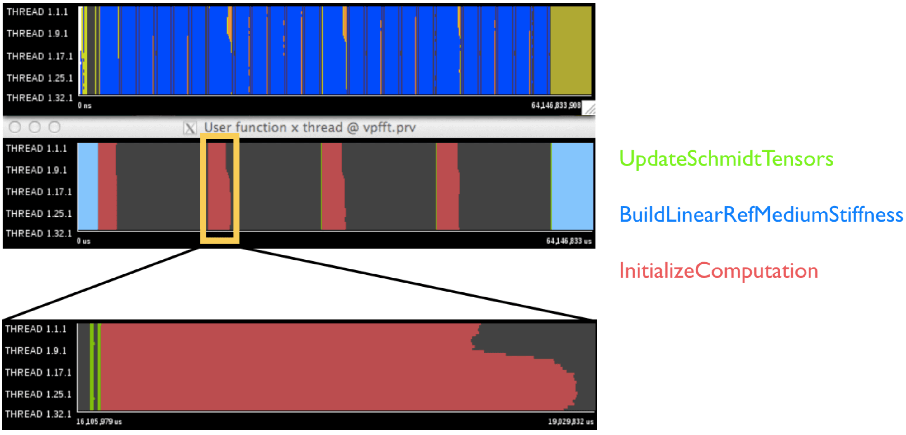
In this section we dive deeper into the code of VPFFT to try and find the possible causes of imbalance caused by the algorithm in the time step initialization phases and try to design potential solutions for the problem. For this, we collect information about the user functions, specifically the ones that are called in the time step initialization phases. This section of the code can be seen in the file Src/MaterialGrid.cpp, on the function MaterialGrid::RunSingleStrainStep. The relevant functions being called before the iterations are UpdateSchmidtTensors, InitializeComputation and BuildLinearRefMediumStiffness. In Figure 13 we can see the results and clearly identify the InitializeComputation function as the region where imbalance occurs. We proceed to check its code and repeat the process - results are shown in Figure 14.
 |
|---|
| Left: User functions for the time step initialization phases. Right: colors identifying which regions correspond to each of the functions. |
 |
|---|
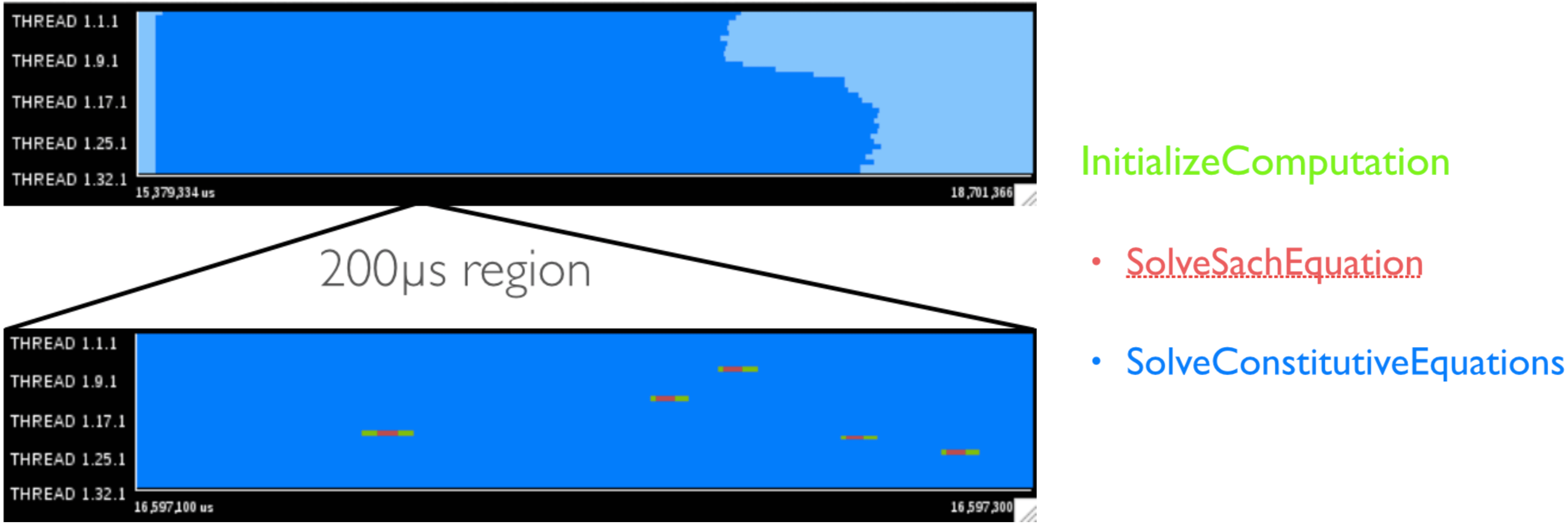
Left: User functions for the InitializeComputation function and direct sub-functions, with a zoomed region of 200µs. Right: colors identifying which regions correspond to each function. |
We can see that most of the time in InitializeComputation is spent in the SolveConstitutiveEquations (over 99%!), and that the function is called multiple times (as shown on the 200µs section), interleaved with SolveSachEquations. Upon closer inspection of the source code for this function, we can see it performs a variable number of iterations, depending of a local error value being under a determined epsilon threashold. This appears to be the cause for imbalance in the time step initialization region. The computation performed inside the loop appears to have similar duration across iterations.
Network conditions
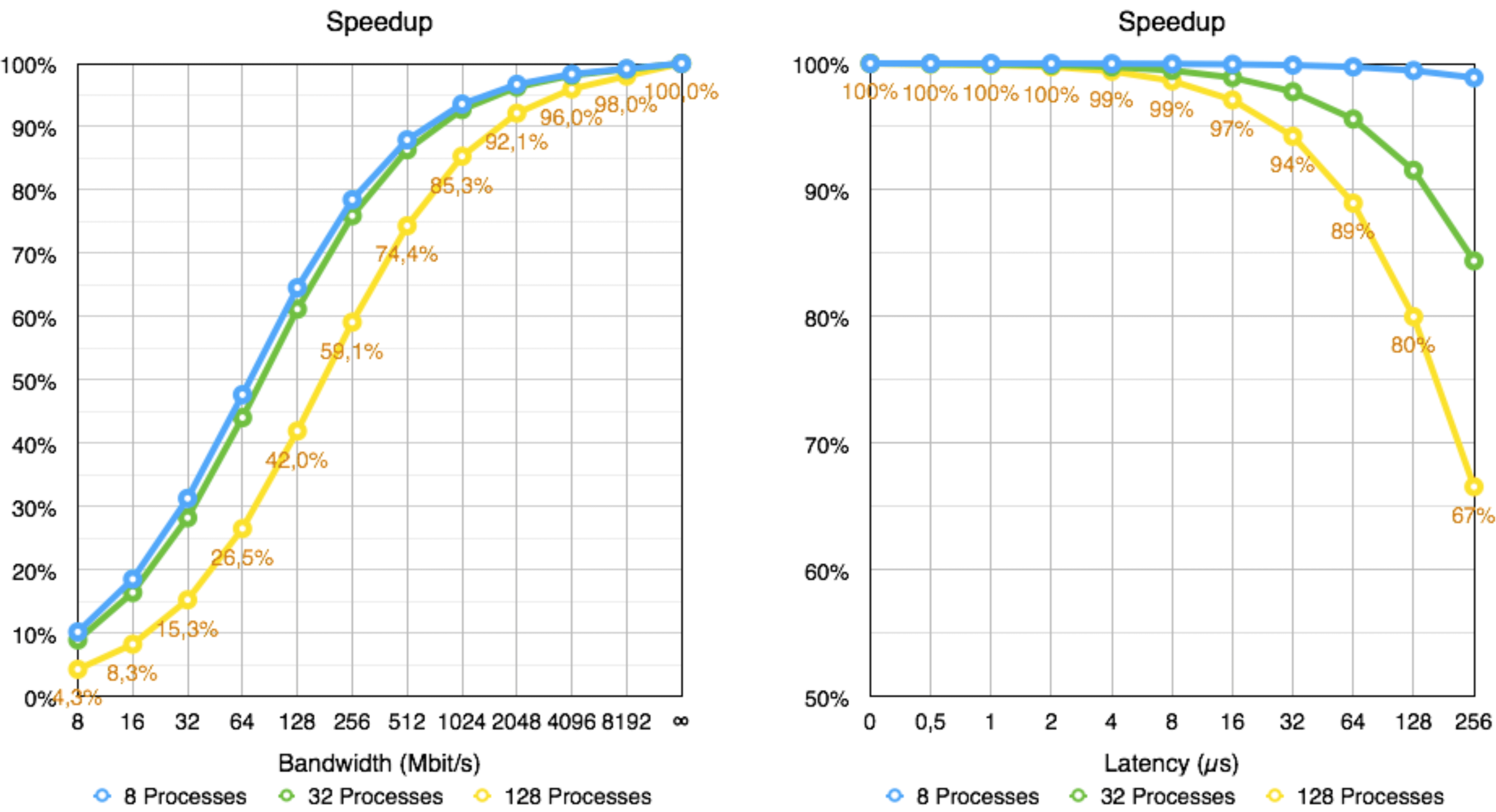
As seen in the efficiency models presented, transfer balance is not an issue at small scales but (very) slowly degrades as we add more processes. In this section we evaluate how network latency and bandwidth might affect the execution of the application. The results obtained can be seen in Figure 15.
 |
|---|
| Speedup for different values of Global bandwidth and End-to-End Latency for 8, 32 and 128 processes. The scale is normalized so that 100% is with an ideal, *perfect network.* |
The application seems to be sensible to bandwidth - there is a rapid decrease from 32 processes to 128 processes and if bandwidth is less than 1Gbps. For today’s supercomputers, this is not an issue, as the global bandwidth exceeds 8Gbps - we expect the application to run very efficiency (over 98%) for 128 processes. As the number of processes is expected to increase, so is the amount of bandwidth required to maintain a constant efficiency ratio.
Regarding latency, there is little impact at this scale - we get over 99.5% speedup with latencies of 2µs or less, which is similar to what exists in today’s machines.
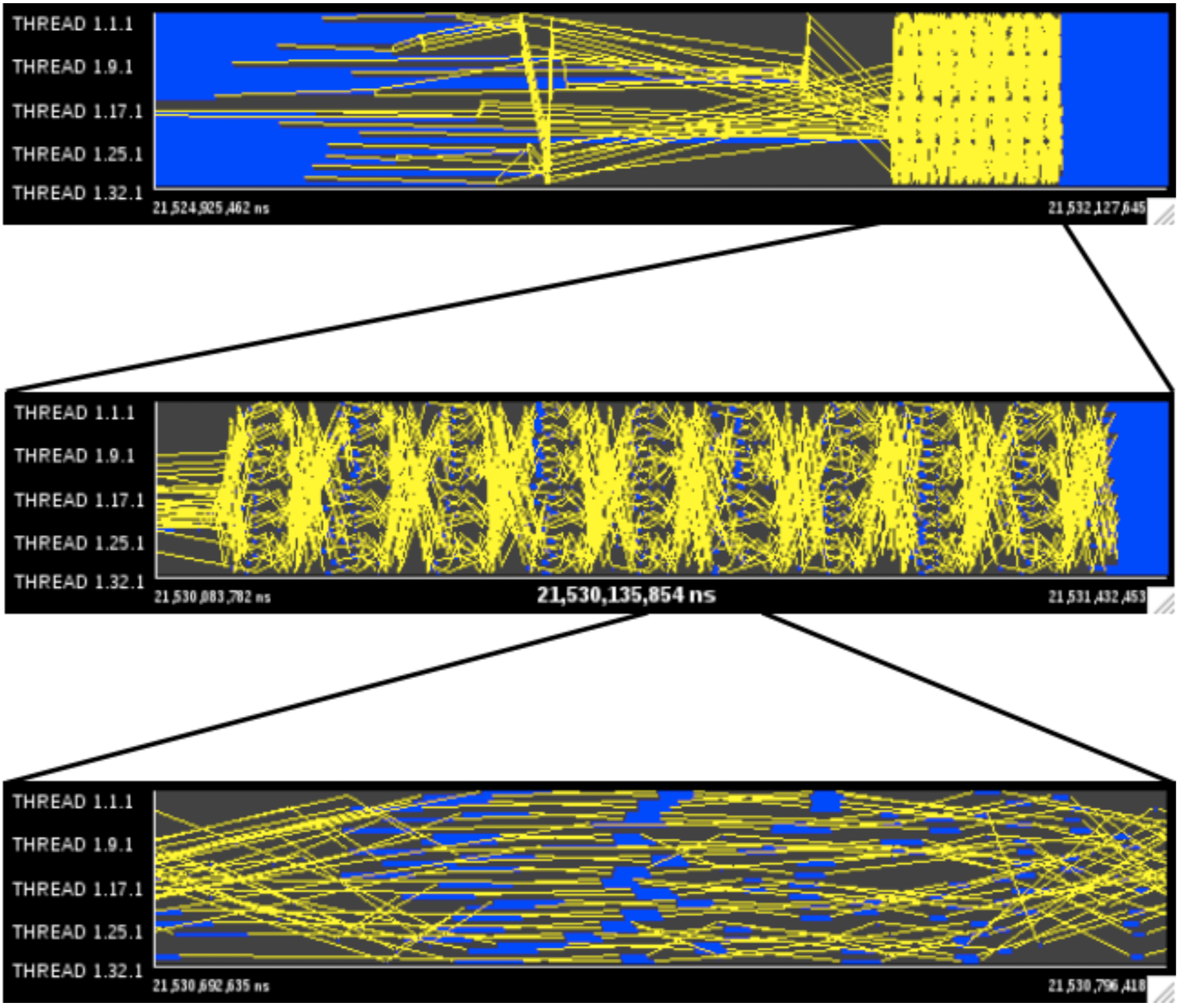
Both factors’ impact mostly the time spent doing MPI SendRecv, with little impact on time spent in AllReduce. As seen before in Figure 5, this means it won’t matter much, as the main problem is the time spent in AllReduce. There appears to be no endpoint contention upon analyzing SendRecv calls - although the communication pattern seems complex, we can see from figure 16 that all processes communicate with a different process.
Speculation about how much speedup from using a certain number of processes is outside the scope of this report, but MareNostrum III’s network is expected to easily support thousands of processes with over 90% efficiency.
 |
|---|
| A perspective on the SendRecv regions’ communication pattern |
Shared memory
The first version of VPFFT++ had support for OpenMP, which was dropped in the current version for MPI. However, VPFFT++ can benefit from both coexisting at the same time. The same methodology of splitting work between processes in MPI can definitely be applied for OpenMP/OmpSS. If algorithm correctness is not invalidated, one can split work in the Y and Z dimensions of the matrix as well, allowing to use more threads for small matrix sizes (which currently cannot be accomplished with current workload distribution granularity).
Conclusion
While not perfect, VPFFT++ appears to scale pretty well! One must note that if running the default number of iterations per time step (100), the time spent in its initialization will account for less than 2% of the total step execution time. Something to look would be alternative ways of solving the constitutive equations, or somehow computing the error globally between all processes - this would cause them to be balanced at the expense of significantly increased communication during this phase. However, this suggestion does not account for the correctness of the algorithm - it might not be feasible at all!
The imbalance caused by TurboBoost is something external to the application that can be worked around. The simplest solution would be to disable it completely, causing all cores to run at the base frequency - this wouldn’t be the best solution, as 20% of the computational power is lost. The best solution would be to make use of all the cores - either by placing more processes in a single node, or by making use of the Shared Memory paradigm by implementing OpenMP or OmpSS. The former would be preferred for regions that are well balanced, while the latter might bring some extra advantages only to the time step initialization phases - this verification was outside the scope of this report.
Regarding the network, it appears to have a limited impact on the application execution time, and endpoint contention is not an issue. MareNostrum III appears to be able to accomodate several thousands of processes without either network bandwidth or latency becoming a significant issue.
The most important improvement would be to make use of all threads in a single machine, so implementation of OpenMP/OmpSS would be of maximum priority.